
-
라이브러리 및 데이터 준비
-
탐색적 자료 분석
-
pd.DataFrame.head()
-
pd.DataFrame.shape
-
pd.DataFrame.info()
-
pd.DataFrame.describe()
-
pd.DataFrame.groupby()
-
matplotlib
-
plt.title(label, fontsize)
-
plt.xlabel(label, fontsize)
-
plt.ylabel(label, fontsize)
-
plt.axvline(x, color)
-
plt.text(x, y, s, fontsize)
-
상관계수
-
pd.DataFrame.corr()
-
3. 데이터 전처리
-
Data Cleansing & Pre-Processing
-
pd.Series.isna()
-
pd.DataFrame.fillna()
-
4. 변수 선택 및 모델 구축
-
model.fit()
-
5. 모델 학습 및 검증
-
randomforestregressor parameter tuning
-
lightgbm parameter tuning
-
xgboost parameter tuning
-
model.predict()
데이콘의 기본 연습대회로 머신러닝에 대해 공부해보았다.
라이브러리 및 데이터 준비
import numpy as np
import pandas as pd
import seaborn as sns
import matplotlib.pyplot as plt
import matplotlib
import mglearn
import joblib
import math

from sklearn.model_selection import train_test_split, validation_curve, cross_val_score, GridSearchCV
from sklearn.neural_network import MLPClassifier
from statsmodels.graphics.tsaplots import plot_acf, acf
from sklearn.linear_model import Ridge,Lasso,ElasticNet, LinearRegression, SGDRegressor, LogisticRegression
from sklearn.preprocessing import PolynomialFeatures, StandardScaler
from sklearn.pipeline import make_pipeline, Pipeline
from sklearn.metrics import confusion_matrix, precision_score, recall_score, f1_score, roc_curve
from sklearn.naive_bayes import GaussianNB, BernoulliNB, MultinomialNB
from sklearn.svm import SVC, SVR
from sklearn.compose import make_column_transformer,ColumnTransformer
import math
from sklearn.ensemble import VotingRegressor, RandomForestRegressor, BaggingRegressor
from sklearn.tree import DecisionTreeRegressor
import sklearn.metrics as metrics
from xgboost import XGBClassifier, XGBRFRegressor, XGBRegressor
from lightgbm import LGBMRegressor

matplotlib.rcParams['font.family']='Malgun Gothic'
plt.rcParams['font.size']=14
matplotlib.rcParams['axes.unicode_minus'] = False
import warnings
warnings.simplefilter('ignore')먼저 사용할 라이브러리와 기타 설정들을 불러와주었다.
탐색적 자료 분석
pd.DataFrame.head()
- 데이터 프레임의 위에서 부터 n개 행을 보여주는 함수
- n의 기본 값(default 값)은 5
train = pd.read_csv('data/train.csv')
test = pd.read_csv('data/test.csv')
submission = pd.read_csv('data/submission.csv')
display(train.head().T, test.head().T)
- id : 날짜와 시간별 id
- hour_bef_temperature : 1시간 전 기온
- hour_bef_precipitation : 1시간 전 비 정보, 비가 오지 않았으면 0, 비가 오면 1
- hour_bef_windspeed : 1시간 전 풍속(평균)
- hour_bef_humidity : 1시간 전 습도
- hour_bef_visibility : 1시간 전 시정(視程), 시계(視界)(특정 기상 상태에 따른 가시성을 의미)
- hour_bef_ozone : 1시간 전 오존
- hour_bef_pm10 : 1시간 전 미세먼지(머리카락 굵기의 1/5에서 1/7 크기의 미세먼지)
- hour_bef_pm2.5 : 1시간 전 미세먼지(머리카락 굵기의 1/20에서 1/30 크기의 미세먼지)
- count : 시간에 따른 따릉이 대여 수
pd.DataFrame.shape
- 데이터 프레임의 행의 개수와 열의 개수가 저장되어 있는 속성(attribute)
print(train.shape)  # (1459, 11)
print(test.shape) # (715, 10)pd.DataFrame.info()
- 데이터셋의 column별 정보를 알려주는 함수
- 비어 있지 않은 값은 (non-null)은 몇개인지?
- column의 type은 무엇인지?
- type의 종류 : int(정수), float(실수), object(문자열), 등등 (date, ...)
train.info()
pd.DataFrame.describe()
숫자형 (int, float) column들의 기술 통계량을 보여주는 함수
기술통계량이란?
- 해당 column을 대표할 수 있는 통계값들을 의미
기술통계량 종류
- count: 해당 column에서 비어 있지 않은 값의 개수
- mean: 평균
- std: 표준편차
- min: 최솟값 (이상치 포함)
- 25% (Q1): 전체 데이터를 순서대로 정렬했을 때, 아래에서 부터 1/4번째 지점에 있는 값
- 50% (Q2): 중앙값 (전체 데이터를 순서대로 정렬했을 때, 아래에서 부터 2/4번째 지점에 있는 값)
- 75% (Q3): 전체 데이터를 순서대로 정렬했을 때, 아래에서 부터 3/4번째 지점에 있는 값
- max: 최댓값 (이상치 포함)
이상치: 울타리 밖에 있는 부분을 이상치라고 정의함
- 아래쪽 울타리: $Q_1$ - $1.5 * IQR$
- 위쪽 울타리: $Q_3$ + $1.5 * IQR$
- $IQR$ = $Q_3 - Q_1$

train.describe()pd.DataFrame.groupby()
- 집단에 대한 통계량 확인
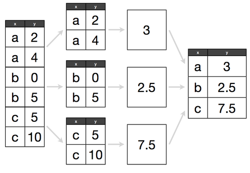
train.groupby(['hour']).count()

train.groupby(['hour']).mean()

train.groupby(['hour'])['count'].mean()

train.groupby(['hour']).mean()['count'].plot()
matplotlib
plt.plot()의 스타일
색깔
| 문자열 | 약자 |
|---|---|
| blue | b |
| green | g |
| red | r |
| cyan | c |
| magenta | m |
| yellow | y |
| black | k |
| white | w |
마커
| 마커 | 의미 |
|---|---|
| . | 점 |
| o | 원 |
| v | 역삼각형 |
| ^ | 삼각형 |
| s | 사각형 |
| * | 별 |
| x | 엑스 |
| d | 다이아몬드 |
선
| 문자열 | 의미 |
|---|---|
| - | 실선 |
| -- | 끊어진 실선 |
| -. | 점+실선 |
| : | 점선 |
plt.plot(train.groupby(['hour']).mean()['count'])
plt.title(label, fontsize)
- 그래프 제목 생성
plt.xlabel(label, fontsize)
- x축 이름 설정
plt.ylabel(label, fontsize)
- y축 이름 설정
plt.plot(train.groupby(['hour']).mean()['count'], 'm*:')
plt.grid()
plt.title('시간 별 따릉이 평균 이용객 수')
plt.xlabel('시간')
plt.ylabel('이용객 수')
plt.axvline(x, color)
- 축을 가로지르는 세로 선 생성
plt.text(x, y, s, fontsize)
- 원하는 위치에 텍스트 생성
plt.plot(train.groupby(['hour']).mean()['count'], 'm*:')
plt.grid()
plt.title('시간 별 따릉이 평균 이용객 수')
plt.xlabel('시간')
plt.ylabel('이용객 수')

plt.axvline(8, color = 'g')
plt.axvline(18, color = 'g')

plt.text(8, 110, '출근')
plt.text(18, 240, '퇴근')
plt.show()
상관계수
- 상관계수: 두 개의 변수가 같이 일어나는 강도를 나타내는 수치
- -1에서 1사이의 값을 가진다.
- -1이나 1인 수치는 현실 세계에서 관측되기 힘든 수치이다.
- 분야별로 기준을 정하는 것에 따라 달라지겠지만, 보통 0.4이상이면 두 개의 변수간에 상관성이 있다고 얘기한다.

- 상관관계는 인과관계와 다르다. 아래의 예시를 확인해보자.
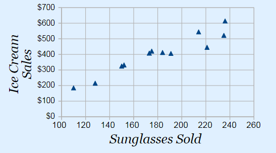
- 선글라스 판매량이 증가함에 따라, 아이스크림 판매액도 같이 증가하는 것을 볼 수 있다.
- 하지만 선글라스 판매량이 증가했기 때문에 아이스크림 판매액이 증가했다라고 해석하는 것은 타당하지 않다.
- 선글라스 판매량이 증가했다는 것은 여름 때문이라고 볼 수 있으므로, 날씨가 더워짐에 따라 선글라스 판매량과 아이스크림 판매액이 같이 증가했다고 보는 것이 타당할 것이다.
pd.DataFrame.corr()
train.corr()plt.figure(figsize = (12, 10))
sns.heatmap(train.corr(), cmap = 'Blues', annot = True, vmin = -1 ,vmax = 1)
plt.show()
3. 데이터 전처리
Data Cleansing & Pre-Processing
pd.Series.isna()
- 결측치 여부를 확인해준다.
- 결측치면 True, 아니면 False
display(train.isna().sum())
display(test.isna().sum())train[train['hour_bef_temperature'].isna()]
결측치가 존재하는 것을 확인할 수 있다.
pd.DataFrame.fillna()
- 결측치를 채우고자 하는 column과 결측치를 대신하여 넣고자 하는 값을 명시해주어야 합니다.
train = pd.read_csv('data/train.csv')
test = pd.read_csv('data/test.csv')

# hour을 기준으로 그룹을 묶는다
a1 = train.groupby('hour')['hour_bef_temperature']
train['hour_bef_temperature'] = a1.apply(lambda x : x.fillna(x.mean()))

b1 = test.groupby('hour')['hour_bef_temperature']
test['hour_bef_temperature'] = b1.apply(lambda x : x.fillna(x.mean()))

# hour_bef_precipitation
a1 = train.groupby('hour')['hour_bef_precipitation']
train['hour_bef_precipitation'] = a1.apply(lambda x : x.fillna(x.mean()))

b1 = test.groupby('hour')['hour_bef_precipitation']
test['hour_bef_precipitation'] = b1.apply(lambda x : x.fillna(x.mean()))

# hour_bef_windspeed
a1 = train.groupby('hour')['hour_bef_windspeed']
train['hour_bef_windspeed'] = a1.apply(lambda x : x.fillna(x.mean()))

b1 = test.groupby('hour')['hour_bef_windspeed']
test['hour_bef_windspeed'] = b1.apply(lambda x : x.fillna(x.mean()))

# hour_bef_humidity
a1 = train.groupby('hour')['hour_bef_humidity']
train['hour_bef_humidity'] = a1.apply(lambda x : x.fillna(x.mean()))

b1 = test.groupby('hour')['hour_bef_humidity']
test['hour_bef_humidity'] = b1.apply(lambda x : x.fillna(x.mean()))

# hour_bef_visibility
a1 = train.groupby('hour')['hour_bef_visibility']
train['hour_bef_visibility'] = a1.apply(lambda x : x.fillna(x.mean()))

b1 = test.groupby('hour')['hour_bef_visibility']
test['hour_bef_visibility'] = b1.apply(lambda x : x.fillna(x.mean()))

# hour_bef_ozone
a1 = train.groupby('hour')['hour_bef_ozone']
train['hour_bef_ozone'] = a1.apply(lambda x : x.fillna(x.mean()))

b1 = test.groupby('hour')['hour_bef_ozone']
test['hour_bef_ozone'] = b1.apply(lambda x : x.fillna(x.mean()))

# hour_bef_pm10
a1 = train.groupby('hour')['hour_bef_pm10']
train['hour_bef_pm10'] = a1.apply(lambda x : x.fillna(x.mean()))

b1 = test.groupby('hour')['hour_bef_pm10']
test['hour_bef_pm10'] = b1.apply(lambda x : x.fillna(x.mean()))

# hour_bef_pm2.5
a1 = train.groupby('hour')['hour_bef_pm2.5']
train['hour_bef_pm2.5'] = a1.apply(lambda x : x.fillna(x.mean()))

b1 = test.groupby('hour')['hour_bef_pm2.5']
test['hour_bef_pm2.5'] = b1.apply(lambda x : x.fillna(x.mean()))

m0 = train[train['hour'] == 0]['hour_bef_ozone'].median()
m2 = train[train['hour'] == 2]['hour_bef_ozone'].median()
train['hour_bef_ozone'].fillna((m0 + m2) / 2, inplace = True)

m0 = test[test['hour'] == 0]['hour_bef_ozone'].median()
m2 = test[test['hour'] == 2]['hour_bef_ozone'].median()
test['hour_bef_ozone'].fillna((m0 + m2) / 2, inplace = True)

m0 = train[train['hour'] == 0]['hour_bef_pm10'].median()
m2 = train[train['hour'] == 2]['hour_bef_pm10'].median()
train['hour_bef_pm10'].fillna((m0 + m2) / 2, inplace = True)

m0 = test[test['hour'] == 0]['hour_bef_pm10'].median()
m2 = test[test['hour'] == 2]['hour_bef_pm10'].median()
test['hour_bef_pm10'].fillna((m0 + m2) / 2, inplace = True)

m0 = train[train['hour'] == 0]['hour_bef_pm2.5'].median()
m2 = train[train['hour'] == 2]['hour_bef_pm2.5'].median()
train['hour_bef_pm2.5'].fillna((m0 + m2) / 2, inplace = True)

m0 = test[test['hour'] == 0]['hour_bef_pm2.5'].median()
m2 = test[test['hour'] == 2]['hour_bef_pm2.5'].median()
test['hour_bef_pm2.5'].fillna((m0 + m2) / 2, inplace = True)

display(train.isna().sum())
display(test.isna().sum())
train['pm10'] = [1 if x <= 30 else 2 if x <= 80 else 3 for x in train['hour_bef_pm10']]
train['pm2.5'] = [1 if x <= 15 else 2 if x <= 35 else 3 for x in train['hour_bef_pm2.5']]

test['pm10'] = [1 if x <= 30 else 2 if x <= 80 else 3 for x in test['hour_bef_pm10']]
test['pm2.5'] = [1 if x <= 15 else 2 if x <= 35 else 3 for x in test['hour_bef_pm2.5']]

train['hour_sin'] = np.sin(2 * np.pi * train['hour']/23.0)
train['hour_cos'] = np.cos(2 * np.pi * train['hour']/23.0)

test['hour_sin'] = np.sin(2 * np.pi * test['hour']/23.0)
test['hour_cos'] = np.cos(2 * np.pi * test['hour']/23.0)

# train.drop('hour', axis = 1, inplace=True)
# test.drop('hour', axis = 1, inplace=True)

display(train.isna().sum())
display(test.isna().sum())train dataset과 teat dataset 모두 동일하게 값들을 설정해주어야 한다.
train_corr = train.drop('id', axis = 1)
plt.figure(figsize = (12, 10))
sns.heatmap(train_corr.corr(), cmap = 'Blues', annot = True, vmin = -1 ,vmax = 1)
plt.show()
from statsmodels.stats.outliers_influence import variance_inflation_factor
train_vif = train_corr.drop(['count', 'pm2.5', 'pm10'], axis = 1)
vif = pd.DataFrame()
vif['VIF Factor']= [ variance_inflation_factor(train_vif.values, i )  for i in range(train_vif.shape[1] ) ]
vif['features'] = train_vif.columns
vif
종속변수인 count와 상관이 있는 변수는 'hour', 'hour_bef_temperature', 'hour_bef_windspeed', 'hour_bef_humidity', 'hour_bef_ozone' 정도로 보인다

각 변수 별 상관계수와 다중공선성을 확인하는 작업이다. 다중공선성이 10 이상이면 독립 변수들 간 강한 상관관계가 나타난다고 할 수 있다. 다중공선성으로 인한 높은 상관관계는 회귀분석의 가정을 위배하고, 종속변수에 안좋은 영향을 미칠 수 있으므로 제거하는 편이 좋다.
train_vif = train_vif.drop('hour_bef_temperature', axis = 1)
# test = test.drop('hour_bef_temperature', axis = 1)
vif = pd.DataFrame()
vif['VIF Factor']= [ variance_inflation_factor(train_vif.values, i )  for i in range(train_vif.shape[1] ) ]
vif['features'] = train_vif.columns
vif
다중공선성이 10이 넘는 변수인 'hour_bef_precipitation' 변수를 제거했다. count 변수와 상관관계는 있지만, 분석에 있어 안좋은 영향을 끼칠 것 같았다.
4. 변수 선택 및 모델 구축
target = train['count']
train_df = train.drop('count', axis = 1)

train_df = train[['hour', 'hour_bef_temperature', 'hour_bef_windspeed', 'hour_bef_precipitation', 'hour_bef_humidity']]
test_df = test[['hour', 'hour_bef_temperature', 'hour_bef_windspeed', 'hour_bef_precipitation', 'hour_bef_humidity']]model.fit()
- 모델 학습
x_train, x_test, y_train, y_test = train_test_split(train_df, target, test_size = 0.2, random_state = 1)

model_ridge = make_pipeline(StandardScaler(), Ridge())
model_lasso = make_pipeline(StandardScaler(), Lasso())
model_lr = make_pipeline(StandardScaler(), LinearRegression())
model_logi = make_pipeline(StandardScaler(), LogisticRegression())
model_dt = make_pipeline(StandardScaler(), DecisionTreeRegressor(random_state = 1))
model_svm = make_pipeline(StandardScaler(), SVR())
model_bagg = make_pipeline(StandardScaler(), BaggingRegressor())
model_rf = make_pipeline(StandardScaler(), RandomForestRegressor())
model_xgb = make_pipeline(StandardScaler(), XGBRegressor())
model_lgb = make_pipeline(StandardScaler(), LGBMRegressor())

model_vote = VotingRegressor(estimators = [('tree', model_dt), ('svm', model_svm), ('xgb', model_xgb),
                                            ('lr', model_lr), ('bagg', model_bagg), ('rf', model_rf)])

                                            model_dt.fit(x_train, y_train)
print('train dt rmse : ', metrics.mean_squared_error(y_train, model_dt.predict(x_train))**0.5)
print('test dt rmse : ', metrics.mean_squared_error(y_test, model_dt.predict(x_test))**0.5)
print()

model_lr.fit(x_train, y_train)
print('train lr rmse : ', metrics.mean_squared_error(y_train, model_lr.predict(x_train))**0.5)
print('test lr rmse : ', metrics.mean_squared_error(y_test, model_lr.predict(x_test))**0.5)
print()

model_xgb.fit(x_train, y_train)
print('train xgb rmse : ', metrics.mean_squared_error(y_train, model_xgb.predict(x_train))**0.5)
print('test xgb rmse : ', metrics.mean_squared_error(y_test, model_xgb.predict(x_test))**0.5)
print()

model_svm.fit(x_train, y_train)
print('train svm rmse : ', metrics.mean_squared_error(y_train, model_svm.predict(x_train))**0.5)
print('test svm rmse : ', metrics.mean_squared_error(y_test, model_svm.predict(x_test))**0.5)
print()

model_vote.fit(x_train, y_train)
print('train voting rmse : ', metrics.mean_squared_error(y_train, model_vote.predict(x_train))**0.5)
print('test voting rmse : ', metrics.mean_squared_error(y_test, model_vote.predict(x_test))**0.5)
print()

model_bagg.fit(x_train, y_train)
print('train bagging rmse : ', metrics.mean_squared_error(y_train, model_bagg.predict(x_train))**0.5)
print('test bagging rmse : ', metrics.mean_squared_error(y_test, model_bagg.predict(x_test))**0.5)
print()

model_rf.fit(x_train, y_train)
print('train rf rmse : ', metrics.mean_squared_error(y_train, model_rf.predict(x_train))**0.5)
print('test rf rmse : ', metrics.mean_squared_error(y_test, model_rf.predict(x_test))**0.5)
print()

model_lgb.fit(x_train, y_train)
print('train lgb rmse : ', metrics.mean_squared_error(y_train, model_lgb.predict(x_train))**0.5)
print('test lgb rmse : ', metrics.mean_squared_error(y_test, model_lgb.predict(x_test))**0.5)
print()
여러 모형 중 점수가 괜찮은 3개의 모형 ( xgboost, random forest, lightgbm ) 사용
- voting은 그리드서치가 매우 쉽지 않으므로 패스..
5. 모델 학습 및 검증
randomforestregressor parameter tuning
n_estimators [default=10]
- 결정트리의 갯수를 지정
- 무작정 트리 갯수를 늘리면 성능 좋아지는 것 대비 시간이 걸릴 수 있음
min_samples_split [default=2]
- 노드를 분할하기 위한 최소한의 샘플 데이터수, 과적합을 제어하는데 사용
- 작게 설정할 수록 분할 노드가 많아져 과적합 가능성 증가
min_samples_leaf [default=1]
- 리프노드가 되기 위해 필요한 최소한의 샘플 데이터수
- min_samples_split과 함께 과적합 제어 용도
- 불균형 데이터의 경우 특정 클래스의 데이터가 극도로 작을 수 있으므로 작게 설정 필요
max_features [default= 'auto' ] >>결정트리에서는 default가 none
- 최적의 분할을 위해 고려할 최대 feature 개수
- int형으로 지정 →피처 갯수 / float형으로 지정 →비중
- sqrt 또는 auto : 전체 피처 중 √(피처개수) 만큼 선정
- log : 전체 피처 중 log2(전체 피처 개수) 만큼 선정
max_depth [default=None]
- 트리의 최대 깊이
- 완벽하게 클래스 값이 결정될 때 까지 분할, 또는 데이터 개수가 min_samples_split보다 작아질 때까지 분할
- 깊이가 깊어지면 과적합될 수 있으므로 적절히 제어 필요
max_leaf_nodes [default=None]
- 리프노드의 최대 개수
model_rfr=make_pipeline(StandardScaler(),RandomForestRegressor())
param_grid={'n_estimators':[100,200,300,400,500],
           'max_depth':[2,3,5,7,10],
           'min_samples_leaf':[3,5],
           'min_samples_split':[3,5,8]}
rfr=RandomForestRegressor()

grid_search=GridSearchCV(estimator=rfr,param_grid=param_grid,cv=3,n_jobs=-1,verbose=1)
grid_search.fit(x_train,y_train)
랜덤포레스트 모델을 사용하여 예측을 해보기 위해 데이터에 알맞는 파라미터를 찾는 방법이 여럿 존재한다.
- 그리드서치
- 랜덤서치
- 베이지안 최적화
그리드서치는 최적의 파라미터를 찾는 과정에서 내가 미리 설정한 파라미터의 값의 배열들을 조합하여 가장 최적의 파라미터를 찾는 방법이다. 그리드서치는 탐색 값의 범위를 넓힐수록 가장 적합한 최적 파라미터를 찾을 가능성이 매우 높아지지만 매우 오래 걸린다는 치명적인 단점이 있다. (언젠가 한번 시도해보길 바란다. 자기전에 서치 돌리고 자고 일어나서도 돌아가고 있는 기이한 현상을...)
랜덤서치는 가능한 모든 조합을 시도하는 대신 무작위한 값을 대입해 최적의 값을 찾아가는 방법이다. 그리드서치보다 시간이 적게 걸리지만 확률적으로 좋은 파라미터나 도출될수도 있고 아닐수도 있다.
베이지안 최적화는 최적의 파라미터를 위주로 탐색하는 작업과 임의의 파라미터를 탐색하는 과정을 반복하여 최적의 파라미터를 탐색하는 기법이다. 그리드 + 랜덤 서치를 조합한 방식인데, 그리드서치보다 상대적으로 시간이 덜 걸리지만, 임의의 파라미터를 잘못 설정할 경우, 시간이 더 오래 걸릴 수 있다.
이번 예측에는 간단한 그리드 서치를 사용해보았다.
grid_search.best_params_

# {'max_depth': 10,
# 'min_samples_leaf': 3,
# 'min_samples_split': 5,
# 'n_estimators': 200}

model_rfr=make_pipeline(StandardScaler(),RandomForestRegressor(max_depth=10,min_samples_leaf=3,min_samples_split=3,n_estimators=200))
model_rfr.fit(train_df, target)
lightgbm parameter tuning
n_estimators [default=10]
- 결정트리의 갯수를 지정
- 무작정 트리 갯수를 늘리면 성능 좋아지는 것 대비 시간이 걸릴 수 있음
max_depth [default=None]
- 트리의 최대 깊이
- 완벽하게 클래스 값이 결정될 때 까지 분할, 또는 데이터 개수가 min_samples_split보다 작아질 때까지 분할
- 깊이가 깊어지면 과적합될 수 있으므로 적절히 제어 필요
min_samples_leaf [default=1]
- 리프노드가 되기 위해 필요한 최소한의 샘플 데이터수
- min_samples_split과 함께 과적합 제어 용도
- 불균형 데이터의 경우 특정 클래스의 데이터가 극도로 작을 수 있으므로 작게 설정 필요
learning_rate
- 각 단계에서 가중치를 줄임으로써 모델을 더 강건하게 만든다.
- 일반적으로 0.01-0.2
model_lgb = make_pipeline(StandardScaler(), LGBMRegressor())
param_grid={'n_estimators':[100, 200, 300, 400, 500],
           'max_depth':[2, 3, 5, 7, 10],
           'min_samples_leaf':[1, 3, 5],
           'learning_rate' : [0.01, 0.05, 0.1, 0.5, 1],}
lgb = LGBMRegressor()

grid_search=GridSearchCV(estimator=lgb,param_grid=param_grid,cv=3,n_jobs=12,verbose=1)
grid_search.fit(x_train,y_train)

grid_search.best_params_
# {'learning_rate': 0.05,
# 'max_depth': 5,
# 'min_samples_leaf': 1,
# 'n_estimators': 100}

model_lgb = make_pipeline(StandardScaler(), LGBMRegressor(learning_rate = 0.05, max_depth = 5, min_samples_leaf = 1, n_estimators = 100))
model_lgb.fit(train_df, target)

xgboost parameter tuning
□ General Parameters : XGBoost의 전반적인 기능을 정의함.
booster [default=gbtree] >> 일반적으로 gbtree의 성능이 낫다.
- gbtree: tree-based models
- gblinear: linear models
silent [default=0]
- 1: 동작 메시지를 프린트하지 않음.
□ Booster Parameters (아래는 gbtree booster 기준으로 정리되어있음.)
eta [default=0.3] => learning_rate
- GBM의 학습 속도와 유사.
- 각 단계에서 가중치를 줄임으로써 모델을 더 강건하게 만든다.
- 일반적으로 0.01-0.2
min_child_weight [default=1] (Should be tuned using CV)
- child의 관측(?)에서 요구되는 최소 가중치의 합
- over-fitting vs under-fitting을 조정하기 위한 파라미터.
- 너무 큰 값이 주어지면 under-fitting.
max_depth [default=6] (Should be tuned using CV)
- 트리의 최대 깊이.
- 일반적으로 3-10
max_leaf_nodes
- 최종 노드의 최대 개수. (max number of terminal nodes)
- 이진 트리가 생성되기 때문에 max_depth가 6이면 max_leaf_nodes는 2^6개가 됨.
gamma [default=0]
- 분할을 수행하는데 필요한 최소 손실 감소를 지정한다.
- 알고리즘을 보수적으로 만든다. loss function에 따라 조정해야 한다.
subsample [default=1]
- 각 트리마다의 관측 데이터 샘플링 비율.
- 값을 적게 주면 over-fitting을 방지하지만 값을 너무 작게 주면 under-fitting.
- 일반적으로 0.5-1
colsample_bytree [default=1]
- 각 트리마다의 feature 샘플링 비율.
- 일반적으로 0.5-1
lambda [default=1] => reg_lambda
- 가중치에 대한 L2 정규화 용어 (Ridge 회귀 분석과 유사(?))
alpha [default=0] => reg_alpha
- 가중치에 대한 L1 정규화 용어 (Lasso 회귀 분석과 유사(?))
scale_pos_weight [default=1]
- 불균형한 경우 더 빠른 수렴(convergence)에 도움되므로 0보다 큰 값을 쓸것.
# grid search
model_xgb = Pipeline( [ ('scl', StandardScaler()), ('xgb', XGBRegressor(n_jobs = 12)) ] )
param_value = {'xgb__n_estimators' : [50, 100, 150, 200, 250, 300],
               'xgb__learning_rate' : [0.01, 0.05, 0.1, 0.5, 1],
               'xgb__max_depth' : list(range(2, 20, 3)),
               'xgb__subsample' : [0.25, 0.5, 0.75, 1],
               'xgb__min_child_weight' : [0.5, 1, 1.5, 2]
              }
gridSearch = GridSearchCV(model_xgb, param_grid = param_value, cv = 5, n_jobs = 12, verbose = 1)
gridSearch.fit(x_train, y_train)model.predict()
- 모델 예측
model_xgb = Pipeline( [ ('scl', StandardScaler()), ('xgb', XGBRegressor(base_score=0.5, booster='gbtree',
                              colsample_bylevel=1, colsample_bynode=1,
                              colsample_bytree=1, gamma=0, gpu_id=-1,
                              importance_type='gain',
                              interaction_constraints='', learning_rate=0.05,
                              max_delta_step=0, max_depth=17, min_child_weight=1.5,
                              monotone_constraints='()',
                              n_estimators=300, n_jobs=12, num_parallel_tree=1,
                              random_state=0, reg_alpha=0, reg_lambda=1,
                              scale_pos_weight=1, subsample=0.5,
                              tree_method='exact', validate_parameters=1,
                              verbosity=None)) ] )
model_xgb.fit(train_df, target)


# 결과 비교 후 사용
submission['count'] = model_rfr.predict(test_df)
submission

submission['count'] = model_lgb.predict(test_df)
submission

submission['count'] = model_xgb.predict(test_df)
submission
데이콘의 기본 연습대회로 머신러닝에 대해 공부해보았다.
라이브러리 및 데이터 준비
import numpy as np
import pandas as pd
import seaborn as sns
import matplotlib.pyplot as plt
import matplotlib
import mglearn
import joblib
import math

from sklearn.model_selection import train_test_split, validation_curve, cross_val_score, GridSearchCV
from sklearn.neural_network import MLPClassifier
from statsmodels.graphics.tsaplots import plot_acf, acf
from sklearn.linear_model import Ridge,Lasso,ElasticNet, LinearRegression, SGDRegressor, LogisticRegression
from sklearn.preprocessing import PolynomialFeatures, StandardScaler
from sklearn.pipeline import make_pipeline, Pipeline
from sklearn.metrics import confusion_matrix, precision_score, recall_score, f1_score, roc_curve
from sklearn.naive_bayes import GaussianNB, BernoulliNB, MultinomialNB
from sklearn.svm import SVC, SVR
from sklearn.compose import make_column_transformer,ColumnTransformer
import math
from sklearn.ensemble import VotingRegressor, RandomForestRegressor, BaggingRegressor
from sklearn.tree import DecisionTreeRegressor
import sklearn.metrics as metrics
from xgboost import XGBClassifier, XGBRFRegressor, XGBRegressor
from lightgbm import LGBMRegressor

matplotlib.rcParams['font.family']='Malgun Gothic'
plt.rcParams['font.size']=14
matplotlib.rcParams['axes.unicode_minus'] = False
import warnings
warnings.simplefilter('ignore')
먼저 사용할 라이브러리와 기타 설정들을 불러와주었다.
탐색적 자료 분석
pd.DataFrame.head()
- 데이터 프레임의 위에서 부터 n개 행을 보여주는 함수
- n의 기본 값(default 값)은 5
train = pd.read_csv('data/train.csv')
test = pd.read_csv('data/test.csv')
submission = pd.read_csv('data/submission.csv')
display(train.head().T, test.head().T)
- id : 날짜와 시간별 id
- hour_bef_temperature : 1시간 전 기온
- hour_bef_precipitation : 1시간 전 비 정보, 비가 오지 않았으면 0, 비가 오면 1
- hour_bef_windspeed : 1시간 전 풍속(평균)
- hour_bef_humidity : 1시간 전 습도
- hour_bef_visibility : 1시간 전 시정(視程), 시계(視界)(특정 기상 상태에 따른 가시성을 의미)
- hour_bef_ozone : 1시간 전 오존
- hour_bef_pm10 : 1시간 전 미세먼지(머리카락 굵기의 1/5에서 1/7 크기의 미세먼지)
- hour_bef_pm2.5 : 1시간 전 미세먼지(머리카락 굵기의 1/20에서 1/30 크기의 미세먼지)
- count : 시간에 따른 따릉이 대여 수
pd.DataFrame.shape
- 데이터 프레임의 행의 개수와 열의 개수가 저장되어 있는 속성(attribute)
print(train.shape)  # (1459, 11)
print(test.shape)    # (715, 10)
pd.DataFrame.info()
- 데이터셋의 column별 정보를 알려주는 함수
- 비어 있지 않은 값은 (non-null)은 몇개인지?
- column의 type은 무엇인지?
- type의 종류 : int(정수), float(실수), object(문자열), 등등 (date, ...)
train.info()
pd.DataFrame.describe()
숫자형 (int, float) column들의 기술 통계량을 보여주는 함수
기술통계량이란?
- 해당 column을 대표할 수 있는 통계값들을 의미
기술통계량 종류
- count: 해당 column에서 비어 있지 않은 값의 개수
- mean: 평균
- std: 표준편차
- min: 최솟값 (이상치 포함)
- 25% (Q1): 전체 데이터를 순서대로 정렬했을 때, 아래에서 부터 1/4번째 지점에 있는 값
- 50% (Q2): 중앙값 (전체 데이터를 순서대로 정렬했을 때, 아래에서 부터 2/4번째 지점에 있는 값)
- 75% (Q3): 전체 데이터를 순서대로 정렬했을 때, 아래에서 부터 3/4번째 지점에 있는 값
- max: 최댓값 (이상치 포함)
이상치: 울타리 밖에 있는 부분을 이상치라고 정의함
- 아래쪽 울타리: $Q_1$ - $1.5 * IQR$
- 위쪽 울타리: $Q_3$ + $1.5 * IQR$
- $IQR$ = $Q_3 - Q_1$
train.describe()pd.DataFrame.groupby()
- 집단에 대한 통계량 확인
train.groupby(['hour']).count()

train.groupby(['hour']).mean()

train.groupby(['hour'])['count'].mean()

train.groupby(['hour']).mean()['count'].plot()
matplotlib
plt.plot()의 스타일
색깔
| 문자열 | 약자 |
|---|---|
| blue | b |
| green | g |
| red | r |
| cyan | c |
| magenta | m |
| yellow | y |
| black | k |
| white | w |
마커
| 마커 | 의미 |
|---|---|
| . | 점 |
| o | 원 |
| v | 역삼각형 |
| ^ | 삼각형 |
| s | 사각형 |
| * | 별 |
| x | 엑스 |
| d | 다이아몬드 |
선
| 문자열 | 의미 |
|---|---|
| - | 실선 |
| -- | 끊어진 실선 |
| -. | 점+실선 |
| : | 점선 |
plt.plot(train.groupby(['hour']).mean()['count'])
plt.title(label, fontsize)
- 그래프 제목 생성
plt.xlabel(label, fontsize)
- x축 이름 설정
plt.ylabel(label, fontsize)
- y축 이름 설정
plt.plot(train.groupby(['hour']).mean()['count'], 'm*:')
plt.grid()
plt.title('시간 별 따릉이 평균 이용객 수')
plt.xlabel('시간')
plt.ylabel('이용객 수')
plt.axvline(x, color)
- 축을 가로지르는 세로 선 생성
plt.text(x, y, s, fontsize)
- 원하는 위치에 텍스트 생성
plt.plot(train.groupby(['hour']).mean()['count'], 'm*:')
plt.grid()
plt.title('시간 별 따릉이 평균 이용객 수')
plt.xlabel('시간')
plt.ylabel('이용객 수')

plt.axvline(8, color = 'g')
plt.axvline(18, color = 'g')

plt.text(8, 110, '출근')
plt.text(18, 240, '퇴근')
plt.show()
상관계수
- 상관계수: 두 개의 변수가 같이 일어나는 강도를 나타내는 수치
- -1에서 1사이의 값을 가진다.
- -1이나 1인 수치는 현실 세계에서 관측되기 힘든 수치이다.
- 분야별로 기준을 정하는 것에 따라 달라지겠지만, 보통 0.4이상이면 두 개의 변수간에 상관성이 있다고 얘기한다.
- 상관관계는 인과관계와 다르다. 아래의 예시를 확인해보자.
- 선글라스 판매량이 증가함에 따라, 아이스크림 판매액도 같이 증가하는 것을 볼 수 있다.
- 하지만 선글라스 판매량이 증가했기 때문에 아이스크림 판매액이 증가했다라고 해석하는 것은 타당하지 않다.
- 선글라스 판매량이 증가했다는 것은 여름 때문이라고 볼 수 있으므로, 날씨가 더워짐에 따라 선글라스 판매량과 아이스크림 판매액이 같이 증가했다고 보는 것이 타당할 것이다.
pd.DataFrame.corr()
train.corr()plt.figure(figsize = (12, 10))
sns.heatmap(train.corr(), cmap = 'Blues', annot = True, vmin = -1 ,vmax = 1)
plt.show()
3. 데이터 전처리
Data Cleansing & Pre-Processing
pd.Series.isna()
- 결측치 여부를 확인해준다.
- 결측치면 True, 아니면 False
display(train.isna().sum())
display(test.isna().sum())train[train['hour_bef_temperature'].isna()]
결측치가 존재하는 것을 확인할 수 있다.
pd.DataFrame.fillna()
- 결측치를 채우고자 하는 column과 결측치를 대신하여 넣고자 하는 값을 명시해주어야 합니다.
train = pd.read_csv('data/train.csv')
test = pd.read_csv('data/test.csv')

# hour을 기준으로 그룹을 묶는다
a1 = train.groupby('hour')['hour_bef_temperature']
train['hour_bef_temperature'] = a1.apply(lambda x : x.fillna(x.mean()))

b1 = test.groupby('hour')['hour_bef_temperature']
test['hour_bef_temperature'] = b1.apply(lambda x : x.fillna(x.mean()))

# hour_bef_precipitation
a1 = train.groupby('hour')['hour_bef_precipitation']
train['hour_bef_precipitation'] = a1.apply(lambda x : x.fillna(x.mean()))

b1 = test.groupby('hour')['hour_bef_precipitation']
test['hour_bef_precipitation'] = b1.apply(lambda x : x.fillna(x.mean()))

# hour_bef_windspeed
a1 = train.groupby('hour')['hour_bef_windspeed']
train['hour_bef_windspeed'] = a1.apply(lambda x : x.fillna(x.mean()))

b1 = test.groupby('hour')['hour_bef_windspeed']
test['hour_bef_windspeed'] = b1.apply(lambda x : x.fillna(x.mean()))

# hour_bef_humidity
a1 = train.groupby('hour')['hour_bef_humidity']
train['hour_bef_humidity'] = a1.apply(lambda x : x.fillna(x.mean()))

b1 = test.groupby('hour')['hour_bef_humidity']
test['hour_bef_humidity'] = b1.apply(lambda x : x.fillna(x.mean()))

# hour_bef_visibility
a1 = train.groupby('hour')['hour_bef_visibility']
train['hour_bef_visibility'] = a1.apply(lambda x : x.fillna(x.mean()))

b1 = test.groupby('hour')['hour_bef_visibility']
test['hour_bef_visibility'] = b1.apply(lambda x : x.fillna(x.mean()))

# hour_bef_ozone
a1 = train.groupby('hour')['hour_bef_ozone']
train['hour_bef_ozone'] = a1.apply(lambda x : x.fillna(x.mean()))

b1 = test.groupby('hour')['hour_bef_ozone']
test['hour_bef_ozone'] = b1.apply(lambda x : x.fillna(x.mean()))

# hour_bef_pm10
a1 = train.groupby('hour')['hour_bef_pm10']
train['hour_bef_pm10'] = a1.apply(lambda x : x.fillna(x.mean()))

b1 = test.groupby('hour')['hour_bef_pm10']
test['hour_bef_pm10'] = b1.apply(lambda x : x.fillna(x.mean()))

# hour_bef_pm2.5
a1 = train.groupby('hour')['hour_bef_pm2.5']
train['hour_bef_pm2.5'] = a1.apply(lambda x : x.fillna(x.mean()))

b1 = test.groupby('hour')['hour_bef_pm2.5']
test['hour_bef_pm2.5'] = b1.apply(lambda x : x.fillna(x.mean()))

m0 = train[train['hour'] == 0]['hour_bef_ozone'].median()
m2 = train[train['hour'] == 2]['hour_bef_ozone'].median()
train['hour_bef_ozone'].fillna((m0 + m2) / 2, inplace = True)

m0 = test[test['hour'] == 0]['hour_bef_ozone'].median()
m2 = test[test['hour'] == 2]['hour_bef_ozone'].median()
test['hour_bef_ozone'].fillna((m0 + m2) / 2, inplace = True)

m0 = train[train['hour'] == 0]['hour_bef_pm10'].median()
m2 = train[train['hour'] == 2]['hour_bef_pm10'].median()
train['hour_bef_pm10'].fillna((m0 + m2) / 2, inplace = True)

m0 = test[test['hour'] == 0]['hour_bef_pm10'].median()
m2 = test[test['hour'] == 2]['hour_bef_pm10'].median()
test['hour_bef_pm10'].fillna((m0 + m2) / 2, inplace = True)

m0 = train[train['hour'] == 0]['hour_bef_pm2.5'].median()
m2 = train[train['hour'] == 2]['hour_bef_pm2.5'].median()
train['hour_bef_pm2.5'].fillna((m0 + m2) / 2, inplace = True)

m0 = test[test['hour'] == 0]['hour_bef_pm2.5'].median()
m2 = test[test['hour'] == 2]['hour_bef_pm2.5'].median()
test['hour_bef_pm2.5'].fillna((m0 + m2) / 2, inplace = True)

display(train.isna().sum())
display(test.isna().sum())
train['pm10'] = [1 if x <= 30 else 2 if x <= 80 else 3 for x in train['hour_bef_pm10']]
train['pm2.5'] = [1 if x <= 15 else 2 if x <= 35 else 3 for x in train['hour_bef_pm2.5']]

test['pm10'] = [1 if x <= 30 else 2 if x <= 80 else 3 for x in test['hour_bef_pm10']]
test['pm2.5'] = [1 if x <= 15 else 2 if x <= 35 else 3 for x in test['hour_bef_pm2.5']]

train['hour_sin'] = np.sin(2 * np.pi * train['hour']/23.0)
train['hour_cos'] = np.cos(2 * np.pi * train['hour']/23.0)

test['hour_sin'] = np.sin(2 * np.pi * test['hour']/23.0)
test['hour_cos'] = np.cos(2 * np.pi * test['hour']/23.0)

# train.drop('hour', axis = 1, inplace=True)
# test.drop('hour', axis = 1, inplace=True)

display(train.isna().sum())
display(test.isna().sum())
train dataset과 teat dataset 모두 동일하게 값들을 설정해주어야 한다.
train_corr = train.drop('id', axis = 1)
plt.figure(figsize = (12, 10))
sns.heatmap(train_corr.corr(), cmap = 'Blues', annot = True, vmin = -1 ,vmax = 1)
plt.show()
from statsmodels.stats.outliers_influence import variance_inflation_factor
train_vif = train_corr.drop(['count', 'pm2.5', 'pm10'], axis = 1)
vif = pd.DataFrame()
vif['VIF Factor']= [ variance_inflation_factor(train_vif.values, i )  for i in range(train_vif.shape[1] ) ]
vif['features'] = train_vif.columns
vif
종속변수인 count와 상관이 있는 변수는 'hour', 'hour_bef_temperature', 'hour_bef_windspeed', 'hour_bef_humidity', 'hour_bef_ozone' 정도로 보인다
각 변수 별 상관계수와 다중공선성을 확인하는 작업이다. 다중공선성이 10 이상이면 독립 변수들 간 강한 상관관계가 나타난다고 할 수 있다. 다중공선성으로 인한 높은 상관관계는 회귀분석의 가정을 위배하고, 종속변수에 안좋은 영향을 미칠 수 있으므로 제거하는 편이 좋다.
train_vif = train_vif.drop('hour_bef_temperature', axis = 1)
# test = test.drop('hour_bef_temperature', axis = 1)
vif = pd.DataFrame()
vif['VIF Factor']= [ variance_inflation_factor(train_vif.values, i )  for i in range(train_vif.shape[1] ) ]
vif['features'] = train_vif.columns
vif
다중공선성이 10이 넘는 변수인 'hour_bef_precipitation' 변수를 제거했다. count 변수와 상관관계는 있지만, 분석에 있어 안좋은 영향을 끼칠 것 같았다.
4. 변수 선택 및 모델 구축
target = train['count']
train_df = train.drop('count', axis = 1)

train_df = train[['hour', 'hour_bef_temperature', 'hour_bef_windspeed', 'hour_bef_precipitation', 'hour_bef_humidity']]
test_df = test[['hour', 'hour_bef_temperature', 'hour_bef_windspeed', 'hour_bef_precipitation', 'hour_bef_humidity']]
model.fit()
- 모델 학습
x_train, x_test, y_train, y_test = train_test_split(train_df, target, test_size = 0.2, random_state = 1)

model_ridge = make_pipeline(StandardScaler(), Ridge())
model_lasso = make_pipeline(StandardScaler(), Lasso())
model_lr = make_pipeline(StandardScaler(), LinearRegression())
model_logi = make_pipeline(StandardScaler(), LogisticRegression())
model_dt = make_pipeline(StandardScaler(), DecisionTreeRegressor(random_state = 1))
model_svm = make_pipeline(StandardScaler(), SVR())
model_bagg = make_pipeline(StandardScaler(), BaggingRegressor())
model_rf = make_pipeline(StandardScaler(), RandomForestRegressor())
model_xgb = make_pipeline(StandardScaler(), XGBRegressor())
model_lgb = make_pipeline(StandardScaler(), LGBMRegressor())

model_vote = VotingRegressor(estimators = [('tree', model_dt), ('svm', model_svm), ('xgb', model_xgb),
                                            ('lr', model_lr), ('bagg', model_bagg), ('rf', model_rf)])

                                            model_dt.fit(x_train, y_train)
print('train dt rmse : ', metrics.mean_squared_error(y_train, model_dt.predict(x_train))**0.5)
print('test dt rmse : ', metrics.mean_squared_error(y_test, model_dt.predict(x_test))**0.5)
print()

model_lr.fit(x_train, y_train)
print('train lr rmse : ', metrics.mean_squared_error(y_train, model_lr.predict(x_train))**0.5)
print('test lr rmse : ', metrics.mean_squared_error(y_test, model_lr.predict(x_test))**0.5)
print()

model_xgb.fit(x_train, y_train)
print('train xgb rmse : ', metrics.mean_squared_error(y_train, model_xgb.predict(x_train))**0.5)
print('test xgb rmse : ', metrics.mean_squared_error(y_test, model_xgb.predict(x_test))**0.5)
print()

model_svm.fit(x_train, y_train)
print('train svm rmse : ', metrics.mean_squared_error(y_train, model_svm.predict(x_train))**0.5)
print('test svm rmse : ', metrics.mean_squared_error(y_test, model_svm.predict(x_test))**0.5)
print()

model_vote.fit(x_train, y_train)
print('train voting rmse : ', metrics.mean_squared_error(y_train, model_vote.predict(x_train))**0.5)
print('test voting rmse : ', metrics.mean_squared_error(y_test, model_vote.predict(x_test))**0.5)
print()

model_bagg.fit(x_train, y_train)
print('train bagging rmse : ', metrics.mean_squared_error(y_train, model_bagg.predict(x_train))**0.5)
print('test bagging rmse : ', metrics.mean_squared_error(y_test, model_bagg.predict(x_test))**0.5)
print()

model_rf.fit(x_train, y_train)
print('train rf rmse : ', metrics.mean_squared_error(y_train, model_rf.predict(x_train))**0.5)
print('test rf rmse : ', metrics.mean_squared_error(y_test, model_rf.predict(x_test))**0.5)
print()

model_lgb.fit(x_train, y_train)
print('train lgb rmse : ', metrics.mean_squared_error(y_train, model_lgb.predict(x_train))**0.5)
print('test lgb rmse : ', metrics.mean_squared_error(y_test, model_lgb.predict(x_test))**0.5)
print()
여러 모형 중 점수가 괜찮은 3개의 모형 ( xgboost, random forest, lightgbm ) 사용
- voting은 그리드서치가 매우 쉽지 않으므로 패스..
5. 모델 학습 및 검증
randomforestregressor parameter tuning
n_estimators [default=10]
- 결정트리의 갯수를 지정
- 무작정 트리 갯수를 늘리면 성능 좋아지는 것 대비 시간이 걸릴 수 있음
min_samples_split [default=2]
- 노드를 분할하기 위한 최소한의 샘플 데이터수, 과적합을 제어하는데 사용
- 작게 설정할 수록 분할 노드가 많아져 과적합 가능성 증가
min_samples_leaf [default=1]
- 리프노드가 되기 위해 필요한 최소한의 샘플 데이터수
- min_samples_split과 함께 과적합 제어 용도
- 불균형 데이터의 경우 특정 클래스의 데이터가 극도로 작을 수 있으므로 작게 설정 필요
max_features [default= 'auto' ] >>결정트리에서는 default가 none
- 최적의 분할을 위해 고려할 최대 feature 개수
- int형으로 지정 →피처 갯수 / float형으로 지정 →비중
- sqrt 또는 auto : 전체 피처 중 √(피처개수) 만큼 선정
- log : 전체 피처 중 log2(전체 피처 개수) 만큼 선정
max_depth [default=None]
- 트리의 최대 깊이
- 완벽하게 클래스 값이 결정될 때 까지 분할, 또는 데이터 개수가 min_samples_split보다 작아질 때까지 분할
- 깊이가 깊어지면 과적합될 수 있으므로 적절히 제어 필요
max_leaf_nodes [default=None]
- 리프노드의 최대 개수
model_rfr=make_pipeline(StandardScaler(),RandomForestRegressor())
param_grid={'n_estimators':[100,200,300,400,500],
           'max_depth':[2,3,5,7,10],
           'min_samples_leaf':[3,5],
           'min_samples_split':[3,5,8]}
rfr=RandomForestRegressor()

grid_search=GridSearchCV(estimator=rfr,param_grid=param_grid,cv=3,n_jobs=-1,verbose=1)
grid_search.fit(x_train,y_train)
랜덤포레스트 모델을 사용하여 예측을 해보기 위해 데이터에 알맞는 파라미터를 찾는 방법이 여럿 존재한다.
- 그리드서치
- 랜덤서치
- 베이지안 최적화
그리드서치는 최적의 파라미터를 찾는 과정에서 내가 미리 설정한 파라미터의 값의 배열들을 조합하여 가장 최적의 파라미터를 찾는 방법이다. 그리드서치는 탐색 값의 범위를 넓힐수록 가장 적합한 최적 파라미터를 찾을 가능성이 매우 높아지지만 매우 오래 걸린다는 치명적인 단점이 있다. (언젠가 한번 시도해보길 바란다. 자기전에 서치 돌리고 자고 일어나서도 돌아가고 있는 기이한 현상을...)
랜덤서치는 가능한 모든 조합을 시도하는 대신 무작위한 값을 대입해 최적의 값을 찾아가는 방법이다. 그리드서치보다 시간이 적게 걸리지만 확률적으로 좋은 파라미터나 도출될수도 있고 아닐수도 있다.
베이지안 최적화는 최적의 파라미터를 위주로 탐색하는 작업과 임의의 파라미터를 탐색하는 과정을 반복하여 최적의 파라미터를 탐색하는 기법이다. 그리드 + 랜덤 서치를 조합한 방식인데, 그리드서치보다 상대적으로 시간이 덜 걸리지만, 임의의 파라미터를 잘못 설정할 경우, 시간이 더 오래 걸릴 수 있다.
이번 예측에는 간단한 그리드 서치를 사용해보았다.
grid_search.best_params_

# {'max_depth': 10,
# 'min_samples_leaf': 3,
# 'min_samples_split': 5,
# 'n_estimators': 200}

model_rfr=make_pipeline(StandardScaler(),RandomForestRegressor(max_depth=10,min_samples_leaf=3,min_samples_split=3,n_estimators=200))
model_rfr.fit(train_df, target)
lightgbm parameter tuning
n_estimators [default=10]
- 결정트리의 갯수를 지정
- 무작정 트리 갯수를 늘리면 성능 좋아지는 것 대비 시간이 걸릴 수 있음
max_depth [default=None]
- 트리의 최대 깊이
- 완벽하게 클래스 값이 결정될 때 까지 분할, 또는 데이터 개수가 min_samples_split보다 작아질 때까지 분할
- 깊이가 깊어지면 과적합될 수 있으므로 적절히 제어 필요
min_samples_leaf [default=1]
- 리프노드가 되기 위해 필요한 최소한의 샘플 데이터수
- min_samples_split과 함께 과적합 제어 용도
- 불균형 데이터의 경우 특정 클래스의 데이터가 극도로 작을 수 있으므로 작게 설정 필요
learning_rate
- 각 단계에서 가중치를 줄임으로써 모델을 더 강건하게 만든다.
- 일반적으로 0.01-0.2
model_lgb = make_pipeline(StandardScaler(), LGBMRegressor())
param_grid={'n_estimators':[100, 200, 300, 400, 500],
           'max_depth':[2, 3, 5, 7, 10],
           'min_samples_leaf':[1, 3, 5],
           'learning_rate' : [0.01, 0.05, 0.1, 0.5, 1],}
lgb = LGBMRegressor()

grid_search=GridSearchCV(estimator=lgb,param_grid=param_grid,cv=3,n_jobs=12,verbose=1)
grid_search.fit(x_train,y_train)

grid_search.best_params_
# {'learning_rate': 0.05,
# 'max_depth': 5,
# 'min_samples_leaf': 1,
# 'n_estimators': 100}

model_lgb = make_pipeline(StandardScaler(), LGBMRegressor(learning_rate = 0.05, max_depth = 5, min_samples_leaf = 1, n_estimators = 100))
model_lgb.fit(train_df, target)
xgboost parameter tuning
□ General Parameters : XGBoost의 전반적인 기능을 정의함.
booster [default=gbtree] >> 일반적으로 gbtree의 성능이 낫다.
- gbtree: tree-based models
- gblinear: linear models
silent [default=0]
- 1: 동작 메시지를 프린트하지 않음.
□ Booster Parameters (아래는 gbtree booster 기준으로 정리되어있음.)
eta [default=0.3] => learning_rate
- GBM의 학습 속도와 유사.
- 각 단계에서 가중치를 줄임으로써 모델을 더 강건하게 만든다.
- 일반적으로 0.01-0.2
min_child_weight [default=1] (Should be tuned using CV)
- child의 관측(?)에서 요구되는 최소 가중치의 합
- over-fitting vs under-fitting을 조정하기 위한 파라미터.
- 너무 큰 값이 주어지면 under-fitting.
max_depth [default=6] (Should be tuned using CV)
- 트리의 최대 깊이.
- 일반적으로 3-10
max_leaf_nodes
- 최종 노드의 최대 개수. (max number of terminal nodes)
- 이진 트리가 생성되기 때문에 max_depth가 6이면 max_leaf_nodes는 2^6개가 됨.
gamma [default=0]
- 분할을 수행하는데 필요한 최소 손실 감소를 지정한다.
- 알고리즘을 보수적으로 만든다. loss function에 따라 조정해야 한다.
subsample [default=1]
- 각 트리마다의 관측 데이터 샘플링 비율.
- 값을 적게 주면 over-fitting을 방지하지만 값을 너무 작게 주면 under-fitting.
- 일반적으로 0.5-1
colsample_bytree [default=1]
- 각 트리마다의 feature 샘플링 비율.
- 일반적으로 0.5-1
lambda [default=1] => reg_lambda
- 가중치에 대한 L2 정규화 용어 (Ridge 회귀 분석과 유사(?))
alpha [default=0] => reg_alpha
- 가중치에 대한 L1 정규화 용어 (Lasso 회귀 분석과 유사(?))
scale_pos_weight [default=1]
- 불균형한 경우 더 빠른 수렴(convergence)에 도움되므로 0보다 큰 값을 쓸것.
# grid search
model_xgb = Pipeline( [ ('scl', StandardScaler()), ('xgb', XGBRegressor(n_jobs = 12)) ] )
param_value = {'xgb__n_estimators' : [50, 100, 150, 200, 250, 300],
               'xgb__learning_rate' : [0.01, 0.05, 0.1, 0.5, 1],
               'xgb__max_depth' : list(range(2, 20, 3)),
               'xgb__subsample' : [0.25, 0.5, 0.75, 1],
               'xgb__min_child_weight' : [0.5, 1, 1.5, 2]
              }
gridSearch = GridSearchCV(model_xgb, param_grid = param_value, cv = 5, n_jobs = 12, verbose = 1)
gridSearch.fit(x_train, y_train)
model.predict()
- 모델 예측
model_xgb = Pipeline( [ ('scl', StandardScaler()), ('xgb', XGBRegressor(base_score=0.5, booster='gbtree',
                              colsample_bylevel=1, colsample_bynode=1,
                              colsample_bytree=1, gamma=0, gpu_id=-1,
                              importance_type='gain',
                              interaction_constraints='', learning_rate=0.05,
                              max_delta_step=0, max_depth=17, min_child_weight=1.5,
                              monotone_constraints='()',
                              n_estimators=300, n_jobs=12, num_parallel_tree=1,
                              random_state=0, reg_alpha=0, reg_lambda=1,
                              scale_pos_weight=1, subsample=0.5,
                              tree_method='exact', validate_parameters=1,
                              verbosity=None)) ] )
model_xgb.fit(train_df, target)


# 결과 비교 후 사용
submission['count'] = model_rfr.predict(test_df)
submission

submission['count'] = model_lgb.predict(test_df)
submission

submission['count'] = model_xgb.predict(test_df)
submission